Algorithm
Dijkstra’s algorithm is an algorithm that finds the shortest paths from a given node (called the source) to all reachable nodes from it in a weighted digraph with positive weights. It was made by Edsger W. Dijkstra in 1956. This algorithm qualifies as a greedy algorithm. Assuming you are already familiar with greedy heuristics, I will just list here the 2 main properties that Dijkstra algorithm must exhibits:
- optimal substructure : in general, the optimal solution of a given problem can be obtain by using optimal solution of its sub-problems. In case of Dijkstra, any sub-path of a shortest path is a shortest-path (similar with Bellman-Ford – see the similarity).
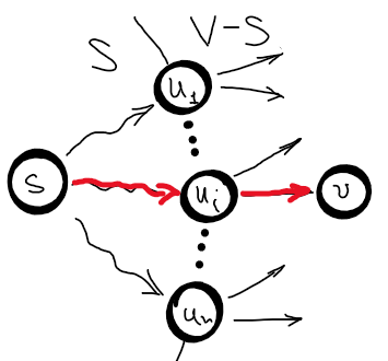
- greedy choice property : make the optimal local choice in the hope of obtaining the global optimum, or in other words, make the best choice at the current moment and then solve the next sub-problems. In case of Dijkstra, let \(S\) be the set of nodes whose shortest distances are already known. Then the estimated distance from \(s \in S\) to \(v \in \left \{ S - V\right \}\) through edge \((u, v)\), where \(u \in S\) is the shortest distance from \(s\) to \(v\) (see the picture below for clarity).
1. Optimal Substructure Proof:
Let \(P\) be the shortest path from \(u\) to \(v\) and \(q\) be a sub-path from \(x\) to \(y\).
Let \(Q^{‘}\) be the shortest path from \(x\) to \(y\).
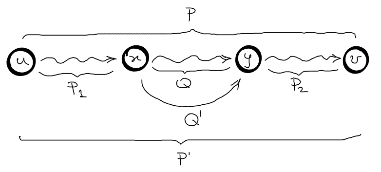
Cut-and-paste: Let’s assume that we can obtain the shortest path \(P\) from \(u\) to \(v\) by using the sub-path \(Q\) which is not the shortest path from \(x\) to \(y\).
\(w(P) = w(P_1) + w(Q) + w(P_2)\)
\(w(P^{'}) = w(P_1) + w(Q^{'}) + w(P_2)\)
\(w(P^{'}) - w(P) = w(Q^{'}) - w(Q)\)
Since \(P\) is the optimal solution, then \(w(P^{'}) - w(P) \leq 0 \Rightarrow w(Q^{'}) \geq w(Q)\), but we know that \(w(Q^{‘}) \leq w(Q)\), so \(w(Q^{‘}) = w(Q)\).
2. Greedy Choice Property Proof:
Let \(S\) be the set of nodes whose shortest path has been discovered.
Let \(u\) be the predecessor of \(v\), where \(u \in S\), \(v \not \in S\) and \(d(u) = \delta (s, u)\).
Assume that \(d(v) = d(u) +w(u, v) \geq \delta (s, v)\) when \(v\) is chosen.
Assume that edge \((x, y)\) is an edge on the shortest path from \(s\) to \(v\) and \(x \in S\) and \(y \not \in S\) and \(d(y) = \delta (s, y)\) since any sub-path of the shortest path is a shortest path.
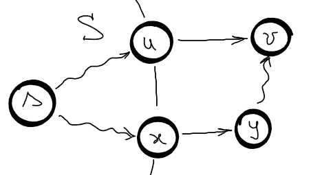
Both \(v\) and \(y\) where in \(V – S\) when \(v\) was chosen, so \(d(v) = d(u) + w(u,v) \leq d(y) = d(x) + w(x, y) = \delta (s, y) \leq \delta(s, v) \Rightarrow d(v) \leq \delta(s, v)\) which is a contradiction.
Implementation
We can implement the algorithm in multiple ways by using different data structures, but let’s keep it simple. We need a way to know which nodes are in \(S\), we need to know the value of the estimate distances and we need a way to make the greedy choice. So, lets use a vector of flags to mark the nodes in S and a vector of ints to keep the estimated distances and to make the greedy choice just traverse the vector with the estimated distances and chose the node \(\not \in S\) with the smallest distance and the other endpoint \(\in S\).
tuple<vector<int>, vector<int>>
	dijkstra(int start, int n, vector<vector<pair<int, int>>>& adjL) {

	vector<bool> s(n, false);
	vector<int> d(n, INF), pred(n);
	d[start] = 0; pred[start] = start;

	for (int k = 1; k <= n; k++) {
		int u = getMin(n, s, d);
		s[u] = true;
		if (d[u] == INF) continue;

		for (pair<int, int> p : adjL[u]) {
			int v = p.first;
			int w = p.second;

			if (s[v] == true) continue;

			if (d[v] > d[u] + w) { // relaxation
				pred[v] = u;
				d[v] = d[u] + w;
			}
		}
	}

	return make_tuple(d, pred);
}

int getMin(int n, vector<bool>& s, vector<int>& d) {
	int v = -1, m = INF;
	for (int u = 0; u < n; u++) {
		if (s[u] == true) continue;
		if (m > d[u]) { v = u; m = d[u]; }
	}

	return v;
}
The greedy choice is made by looping the vector of nodes, which means the time complexity for that is \(O(V)\). So, we can use an adaptive min-priority queue to select the shortest estimated distance and to update the remaining estimated shortest paths, thus the time complexity become logarithmic. But std library of C++ doesn’t support an adaptive min-priority queue (neither Java for what’s worth). However, we can use red-black trees to preserve the logarithmic complexity and for example in C++ we can use multiset. So, whenever we choose a node, we remove that from multiset, and since is a red-black tree, the complexity is logarithmic. And, whenever we need to update the estimated distances, we need to remove a node from the tree and re-inserted with the new distance as priority – still logarithmic. Problem solved, see below an implementation.
tuple<vector<int>, vector<int>>
	dijkstra(int start, int n, vector<vector<pair<int, int>>>& adjL) {

	vector<bool> s(n, false);
	vector<int> d(n, INF), pred(n);
	d[start] = 0; pred[start] = start;

	// min "priority queue" or (x, d=priority)
	struct compare {
		bool operator()(const pair<int, int>& a, const pair<int, int>& b) const {
			return (a.second < b.second);
		}
	};

	// red-black tree: node (x, d=priority)
	multiset <pair<int, int>, compare> rbt;
	for (int u = 0; u < n; u++)
		rbt.insert(make_pair(u, d[u]));

	while (!rbt.empty()) {
		int u = rbt.begin()->first; // top: (x, priority)
		rbt.erase(rbt.begin()); // pop
		s[u] = true;
		if (d[u] == INF) continue;

		for (pair<int, int> p : adjL[u]) {
			int v = p.first;
			int w = p.second;

			if (s[v] == true) continue;
			if (d[v] > d[u] + w) { // relaxation
				rbt.erase(rbt.find(make_pair(v, d[v]))); // delete: log complexity

				pred[v] = u;
				d[v] = d[u] + w;

				rbt.insert(make_pair(v, d[v])); // insert: log complexity
			}
		}
	}

	return make_tuple(d, pred);
}
Example
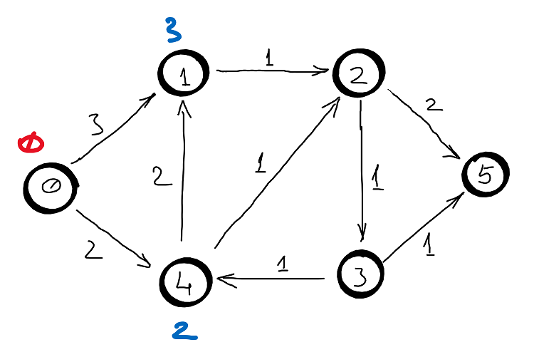
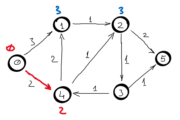
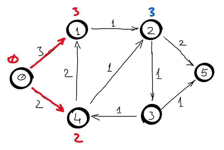
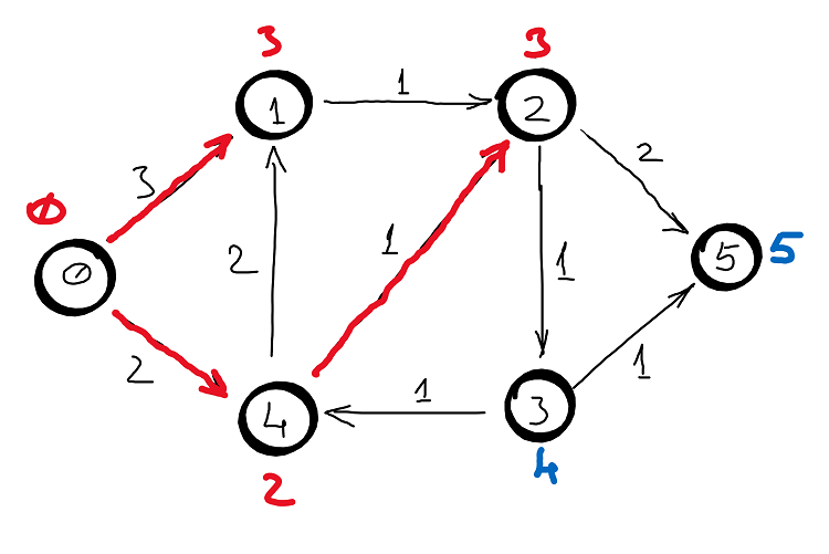
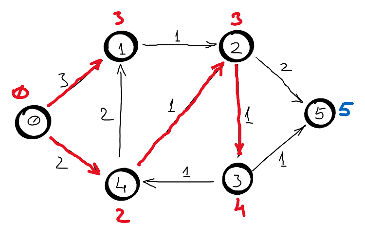
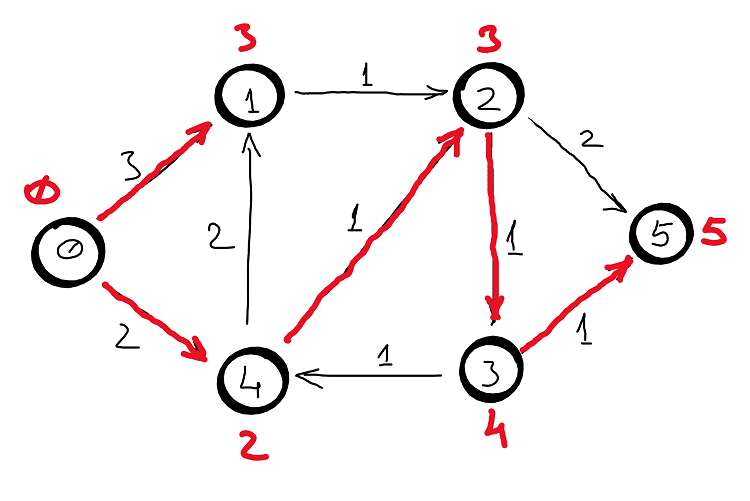
Correctness
Induction hypothesis: assume that \(d(u) = \delta (s, u)\) for all \(u \in S\) and \(d(v)\) are the estimated shortest distances for all \(v \not \in S\).
Base case: \(d(s) = 0\) (the hypothesis obviously holds).
Inductive step: assume \(d(u) = \delta (s, u)\) for all \(u \in S\) and \(d(v)\) are the estimated shortest distances for all \(v \not \in S\) and prove that the estimated shortest distance \(d(v)\) is the shortest distance.
Basically, it is immediately proven by the greedy choice property (see above): \(min \left \{ d(v) = d(u) + w(u, v) \right \} = \delta (s, v)\).
Complexity
\(\sum_{v \in V}degree(v) = 2E\) (1) , graphs (Handshaking Lemma)
\(\sum_{v \in V}degree(v) = E\) (2) , digraphs
looping version
\(T(V,E) = \sum_{v \in V}\left( T_{getMin} + degree(v) \right )\stackrel{(1, 2)}{=} O(V^{2})\)
std::multiset version
Each node is removed from the multiset once, and since each removal is logarithmic, then we have \(\sum_{v \in V} log(V) = O(Vlog (V))\). For each removed node from multiset, the estimated distances through the incident edges are updated (i.e. removed and added again with the new distance), so we have \(\sum_{v \in V} \left( degree(v) 2 log(V) \right ) \stackrel{(1, 2)}{=} O( 2Elog(V)) = O(Elog(V))\).
Therefore, the time complexity is \(T(V, E) = O(Vlog (V) + Elog(V)) = O((V+E)log(V))\).
The auxiliary space complexity is: \(S(V, E) = O(V)\) .
Dijkstra and Negative Weights
Let’s assume we have the following graph.
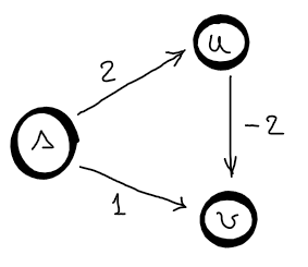
Dijkstra is not working with negative weights, because it assumes that an edge can only increase the distance from the source. So, regarding this graph, the first visited node is \(s\) and update the estimated distances to \(d(u) = 2\) and \(d(v) = 1\). The second visited node is \(v\), after which no other estimated distance is updated since there is no leaving edge from \(v\). Third visited node is \(u\) and since \(v\) is already visited, no estimated distance is updated. So, the distances found by Dijkstra are \(2\) and \(1\) instead of \(2\) and \(0\). You can also look at this from the greedy choice perspective, you cannot reconsider a choice that has been made in the past. So, if there is a negative edge, then you need to reconsider a previous visited node, which violates the greedy choice property.