• Algorithm
  • Implementation
  • Example
• Correctness
• Complexity
• Miscellaneous (the memoization version)

Algorithm

Bellman-Ford is an algorithm that finds the shortest paths from a given node (called the source) to all reachable nodes from it in a weighted digraph without negative cycles. Although it was designed to work on digraph, it works on graphs if each edge is replaced with 2 directional edges of the same weight and opposite direction. But, if an edge has negative weight, then replacing it with directed edges forms a negative cycle and the algorithm fails.

• weighted graphs: \(weights \in R^{+}\)
• weighted digraphs: \(weights \in R\), no negative cycles

The algorithm uses the dynamic programming (DP) optimization method invented by Richard Bellman in 1950. Assuming you are already familiar with dynamic programming, I will just list here the 2 main properties that Bellman-Ford algorithm must exhibits:

• optimal substructure : in general, the optimal solution of a given problem can be obtain by using optimal solution of its sub-problems, in this case any sub-path of a shortest path is a shortest-path
• overlapping subproblems : the recursive algorithm visits the same subproblems repeatedly

Now, lets try to build the recursive DP formula. Let’s assume we already know all the shortest paths from source node \(s\) to all predecessors \(u\) of a node \(v\) and we want to calculate the shortest distance to this node \(v\). Since, we do not know which predecessor is on the shortest path to \(v\) we try them all (classic DP method: I just remembered a cool saying from Erik Demaine “dynamic programming is brute-force done carefully”): \(d(v) = {min}_{u \in V}\left \{ d(u) + w(u, v) \right \}\)

Lets see if this recursivity works. Let’s assume we have the following graph (where 1 is the source node):

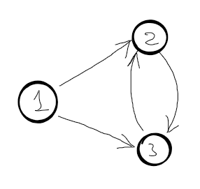
\(d[2]=min\begin{cases} d[1] + w(1,2) \\ d[3] + w(3, 2) \end{cases} \quad d[3]=min\begin{cases} d[1] + w(1, 3) \\ d[2] + w(2, 3) \end{cases} \quad\)

So, there is a circular dependency, which means the algorithm never ends. This is a good example of optimal substructure property violation. This recursive function would work if the graph were a DAG (Direct Acyclic Graph). Another interesting fact, we know that topological sort is possible iff the graph is a DAG, so when we are trying to find the right recursive formula, we actually sort the subproblem topologically.

There is a method to transform any graph in a DAG, by adding the number of edges used in shortest paths.

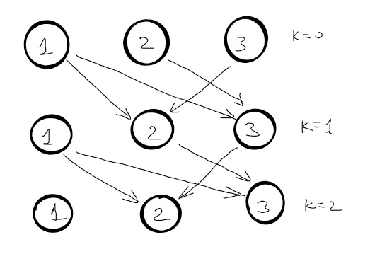
\(d^{k}[2]=min\begin{cases} d^{k-1}[1] + w(1,2) \\ d^{k-1}[3] + w(3, 2) \end{cases} \quad d^{k}[3]=min\begin{cases} d^{k-1}[1] + w(1, 3) \\ d^{k-1}[2] + w(2, 3) \end{cases} \quad\)

Problem solved.

Now, the shortest distance from node \(s\) to node \(v\) can have at most \(V - 1\) edges, where \(V\) is the number of nodes in the graph. If there is a path shorter with multiple edges it means that at least one node is visited more than once and we have a negative cycle. So, for each node we need to find the shortest path that contains at most \(V - 1\). The correct recursive function is: \(d^{k}[v]=min_{u \in V}\begin{cases} 0 & \text{if } v = s \\ \infty & \text{if } v \neq s, k = 0 \\ d^{k-1}[u] + w(u ,v) & \text{otherwise } \\ \end{cases} \quad\)

Implementation

tuple<bool, vector<int>, vector<int>>
	bellmanFord(int source, int n, vector<vector<int>>& edges) {

	bool cycles = false;
	vector<int> d(n, INF), p(n); // distance, predecessor

	d[source] = 0;
	for (int k = 1; k <= n - 1; k++) {
		for (vector<int> e : edges) {
			int u = e[0], v = e[1], w = e[2];

			if (d[u] != INF && d[v] > d[u] + w) { // relaxation
				d[v] = d[u] + w;
				p[v] = u;
			}
		}
	}

	// check negative cycles
	for (vector<int> e : edges) {
		int u = e[0], v = e[1];
		int w = e[2];
    
		if (d[u] != INF && d[v] > d[u] + w) {
			cycles = true; break;
		}
	}

	return make_tuple(cycles, d, p);
}

tuple<bool, vector<int>>
	bellmanFord(int start, int n, vector<vector<pair<int, int>>>& adjL) {

	bool cycle = false;
	vector<int> d(n, INF);
	d[start] = 0;

	for (int k = 1; k <= n - 1; k++) {
		for (int u = 0; u < n; u++) {
			if (d[u] == INF) continue;

			for (pair<int, int> p : adjL[u]) {
				int v = p.first;
				int w = p.second;

				d[v] = min(d[v], d[u] + w); // relaxation
			}
		}
	}

	// check for cycles
	for (int u = 0; u < n; u++) {
		if (d[u] == INF) continue;

		for (pair<int, int> p : adjL[u]) {
			int v = p.first;
			int w = p.second;
			if (d[v] > d[u] + w) {
				cycle = true; break;
			}
		}

		if (cycle) break;
	}

	return make_pair(cycle, d);
}

There is one more trick… when we implement the dynamic programming using tabulation the second dimension of the table is redundant since the shortest distances are built incremental. The side effect is that some distances will be updated faster. In case of memoization the second dimension is required. I will implement this version as well for fun.

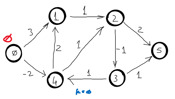
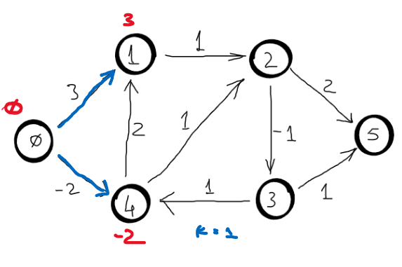
Example

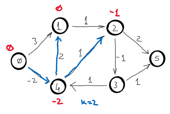
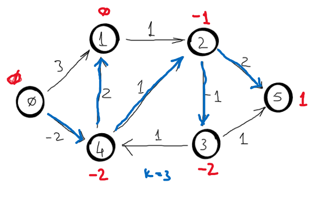
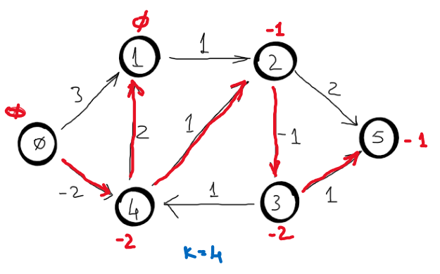
Correctness

Note: The following proof-sketch is based on stanford’s lecture. The proof from CLRS, 3rd edition, pg.653, (Theorem 24.4) is the best alternative.

To be prooved:

1. the algorithm detects negative cycles
2. the algorithm computes correctly the shortest paths after \(V-1\) interations if the graph has no negative cycle

1. Detects negative cycles

Assume that the algorithm finds the shortest path after \(V-1\) iterations, thus \(d^{V-1}{v_i} = \delta(s, v_i)\).
Assume \(v_0, v_1, ..., v_k\) is a negative cycle and \(v_0 = v_k\). This means that \(\sum_{i=1}^{k}w(v_{i-1}, v_i) < 0\).
Assume that the distance to any node \(v_i\) can still be improved after \(V – 1\) iterations, but since the algorithm finds the shortest path in \(V-1\) iterations, we have the following inequality: \(d^{V-1}(v_i) \leq d^{V-1}(v_{i-1}) + w(v_{i-1}, v_i)\).
Adding these inequalities, we get \(\sum_{i=1}^{k}d^{V-1}(v_i) \leq \sum_{i=1}^{k}d^{V-1}(v_{i-1}) + \sum_{i=1}^{k}w(v_{i-1}, v_i)\). The \(\sum_{i=1}^{k}d^{V-1}(v_i) = \sum_{i=1}^{k}d^{V-1}(v_{i-1})\), because \(d^{V-1}(v_0)=d^{V-1}(v_k)\). This basically means that \(\sum_{i=1}^{k}w(v_{i-1}, v_i) \geq 0\) which contradicts the assumption.

2. Computes correctly the shortest paths

Prove by induction on \(k\) that \(d^k(v) = \delta^k(s, v)\) for all \(v \in V\), which means that \(d^{V-1}(v) = \delta(s, v)\).
Induction hypothesis: assume that \(d^{k-1}(v) = \delta^{k-1}(s, v)\) for all \(v \in V\).
Base case: if \(k =0\), then \(d^k(v) = 0\) otherwise \(d^k(v) = \infty\) (the hypothesis obviously holds).
Inductive step: assume \(d^{k-1}(v) = \delta^{k-1}(s, v)\) for all \(v \in V\) and prove that the hypothesis holds for \(d^k(v) = \delta^k(s, v)\)
Let \(P\) be the shortest path from \(s\) to \(v\) that uses at most \(k\) edges. Basically, it means that \(w(P)= \delta^k(s, v)\).
Let \(Q\) be the path from \(s\) to \(u\), where \(u\) is the predecessor of \(v\) on path \(P\). Since shortest paths are composed by shortest paths, then \(Q = \delta^k(s, u)\).
At iteration \(k\) the algorithm does: \(d^k(v) = min \left \{ d^{k-1}(v), d^{k-1}(u) + w(u, v) \right \}\). We know that \(d^{k-1}(v) = \delta^{k-1}(s, v)\) and \(d^{k-1}(u) = \delta^{k-1}(s, u)\) by induction hypothesis. We also know that \(w(P) = w(Q) + w(u, v) = \delta^{k-1}(s, u) + w(u, v) = \delta^k(s, v)\). This means that \(d^k(v) = min \left \{ \delta^{k-1}(s, v), \delta^k(s, v) \right \} = w(P)\). So, the hypothesis holds.

Complexity

Time complexity is quite simple to see: \(T(V, E) = O(V \cdot E)\). For dense graphs (\(E \sim V^2\)) the time complexity is \(T(V, E) = O(V^3)\).
Auxiliary space complexity is \(S(V, E) = O(V)\).

Miscellaneous (the memoization version)

When the tabulation method is used, the distances to each node are constructed by incrementing the number of the maximum number of edges used, but the when the memoization method is used the distances are arbitrary. So, for memoization we need the second dimension for dp table. Here is a trivial example, however it is useful to clear any doubt.

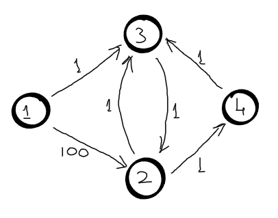
Let node \(1\) be the source node. Let’s assume that the first recursive call visits nodes in this order: \(3 (k=3), 4(k=2), 2(k=1), 1(k=0)\). Now, the \(d[2] = 100\).
\(d^{3}[3]=min\begin{cases} d^{2}[4] + 1 \\ ... \end{cases}\) \(d^{2}[4]=min\begin{cases} d^{1}[2] + 1 \\ ... \end{cases}\) \(d^{1}[2]=d^{0}[1] + 100 = 100\)
Now, let’s assume that the second recursive call visits nodes in this order: \(3 (k=3), 2(k=2), 1(k=1)\). When node \(2\) is visited again, its distance is \(d[2] = 100\), which is not the shortest path from \(1\) to \(2\) using \(2\) edges.

Here is a cpp implementation of the algorithm using memoization:

vector<int> bellmanFordr(int source, int n,
		vector<vector<pair<int, int>>>& adjL) {

	// build incidence list
	vector<vector<pair<int, int>>> incL(n, vector<pair<int, int>>());
	for (int u = 0; u < n; u++) {
		for (pair<int, int> t : adjL[u]) {
			int v = t.first;
			int w = t.second;

			incL[v].push_back(make_pair(u, w));
		}
	}

	vector<vector<int>> d(n, vector<int>(n, INF));
	for (int k = 0; k < n; k++) d[k][source] = 0;

	for (int v = 0; v < n; v++) {
		if (v == source) continue;

		ssspr(source, v, n, n - 2, incL, d);
	}

	return d[n-2];
}

int BFordr(int source, int v, int n, int k,
		vector<vector<pair<int, int>>>& incL,
		vector<vector<int>>& d) {

	if (v == source) return d[k][v];
	if (k == 0) return INF;
	if (d[k][v] != INF) return d[k][v];

	for (pair<int, int> t : incL[v]) {
		int u = t.first;
		int w = t.second;

		int len = ssspr(source, u, n, k - 1, incL, d);
		if (len == INF) continue;

		d[k][v] = min(d[k][v], len + w);
	}

	return d[k][v];
}