- Algorithm
- First Implementation
- Second Implementation (improved time complexity)
- Negative Cycle Detection
Algorithm
Bellman-Ford find the simple shortest path from a single source to all reachable nodes from that source in a weighted digraph with no-negative cycles. It does it by updating the estimated shortest path using at most \(k\) intermediary edges for all \(k\) from \(0\) to \(V-1\), basically \(d^{k}[v]=min_{u \in V} \left \{ d^{k-1}[u] + w(u ,v) \right \} = \delta^{k} (s, v)\) and \(d^{V-1}[u] = \delta(s, v)\).
We can find all-pairs simple shortest paths using same idea, by defining the estimated shortest distance between any two nodes using at most \(k\) edges as:
\(d^{k}(u,v) = min_{x \in V} \left \{ d^{k-1}(u, v), d^{k-1}(u,x) + w(x,v) \right \}\)
\(d^{0}(u,v)=\begin{cases}
0 & \text{if } u = v \\
\infty & \text{otherwise }
\end{cases} \quad\)
\(d^{V-1}(u,v)=\delta(u, v)\)
First Implementation
vector<vector<int>> apspBFord(int n, std::vector<std::vector<int>>& adjM) {

	vector<vector<int>> d(n, vector<int>(n, INF));
	for (int u = 0; u < n; u++) d[u][u] = 0;

	for(int k = 1; k <= n - 1; k++) {

		for (int u = 0; u < n; u++) {
			for (int v = 0; v < n; v++) {

				for (int x = 0; x < n; x++) { // all predecessors of v
					if (adjM[x][v] == INF) continue; // x is not predecessor of v
					if (d[u][x] == INF) continue; // no path from u to x

					d[u][v] = min(d[u][v] , d[u][x] + adjM[x][v]);
				}
			}
		}

	return d;
}
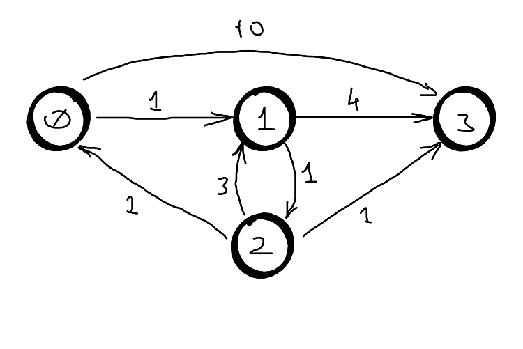
Example

| k=0 | 0 | 1 | 2 | 3 |
|---|---|---|---|---|
| 0 | 0 | inf | inf | inf |
| 1 | inf | 0 | inf | inf |
| 2 | inf | inf | 0 | inf |
| 3 | inf | inf | inf | 0 |
| k=1 | 0 | 1 | 2 | 3 |
|---|---|---|---|---|
| 0 | 0 | 1 | inf | 10 |
| 1 | inf | 0 | 1 | 4 |
| 2 | 1 | 3 | 0 | 1 |
| 3 | inf | inf | inf | 0 |
| k=2 | 0 | 1 | 2 | 3 |
|---|---|---|---|---|
| 0 | 0 | 1 | 2 | 5 |
| 1 | 2 | 0 | 1 | 2 |
| 2 | 1 | 2 | 0 | 1 |
| 3 | inf | inf | inf | 0 |
| k=3 | 0 | 1 | 2 | 3 |
|---|---|---|---|---|
| 0 | 0 | 1 | 2 | 3 |
| 1 | 2 | 0 | 1 | 2 |
| 2 | 1 | 2 | 0 | 1 |
| 3 | inf | inf | inf | 0 |
Note: Just as for classic Bellman-Ford the third dimension is redundant (i.e \(k\)-dimension) for the same reason.
Path Reconstruction
The path can be reconstructed in two ways: by using the previous of the endpoint in current path or by using the next of the start point in current path. There is not much difference between them, but it depends on what problem you need to solve.
For exemplification, let’s consider the path from \(0\) to \(3\) in the above graph: \(0 \rightarrow 1 \rightarrow 2 \rightarrow 3\).
Path reconstruction by predecessors:
- path(0, 3) : 2
- path(0, 2) : 1
- path(0, 1) :0
- path(0, 0) : 0
- Done
Path reconstruction by nexts: - next(0, 3): 1
- next(1, 3): 2
- next(2, 3): 3
- next(3, 3): 3
- Done
I think it is clear by now how this works, however here is the implementation:
tuple < bool, vector<vector<int>>, vector<vector<int>>, vector<vector<int>>>
	apspBFord(int n, std::vector<std::vector<int>>& adjM) {

	vector<vector<int>> d(n, vector<int>(n, INF)),
		pred(n, vector<int>(n, -1)),
		next(n, vector<int>(-1, INF));

	for (int u = 0; u < n; u++) { d[u][u] = 0; pred[u][u] = u; }
	for (int u = 0; u < n; u++)
		for (int v = 0; v < n; v++)
			if (adjM[u][v] != INF) next[u][v] = v;

	for(int k = 1; k <= n - 1; k++) {

		for (int u = 0; u < n; u++) {
			for (int v = 0; v < n; v++) {

				for (int x = 0; x < n; x++) { // all predecessors of v
					if (adjM[x][v] == INF) continue; // x is not predecessor of v
					if (d[u][x] == INF) continue; // no path from u to x

					if (d[u][v] > d[u][v] + adjM[x][v]) {
						d[u][v] = d[u][v] + adjM[x][v];
						pred[u][v] = x;
						next[u][v] = next[u][x];
					}
				}
			}
		}

	return make_tuple(d, pred, next);
}

void predsPath(vector<vector<int>>& path) {
	for (int u = 0; u < n; u++) {
		for (int v = 0; v < n; v++) {
			if (path[u][v] == -1) {
				cout << "   " << setw(4) << " ( INF ) " << u << "->" << v << ": no path " << endl;
				continue;
			}

			cout << "   " << " (" << setw(4) << d[u][v] <<  " ) " << u << "->" << v << ": ";

			int x = u, y = v;
			while (x != y) {
				cout << y << ", ";
				y = path[x][y];
			}
			cout << y << endl;
		}
	}
}

void nextsPath(vector<vector<int>>& path) {
	for (int u = 0; u < n; u++) {
		for (int v = 0; v < n; v++) {
			if (path[u][v] == -1) {
				cout << "   " << setw(4) << " ( INF ) " << u << "->" << v << ": no path " << endl;
				continue;
			}

			cout << "   " << " (" << setw(4) << d[u][v] <<  " ) " << u << "->" << v << ": ";

			int x = u, y = v;
			while (x != y) {
				cout << x << ", ";
				x = path[x][y];
			}
			cout << x << endl;
		}
	}
}
Note: For the nexts the initial table must contain the first endpoint, otherwise it will stuck at the initial node.
Complexity
Time complexity is obvious because of the 4 loops: \(T(V, E) = O(V^4)\), and the auxiliary space complexity \(S(V,E) = O(V^2)\).
Second Implementation (improved time complexity)
We can improve the time complexity of the algorithm by computing only \(log(n)\) distance matrices. Assuming the graph does not contain negative cycle, just as for Bellman-Ford, \(d^{V-1} = d^{V} = d^{V+1}=…\), so if we initialize the first table \(d^1=W\) (where \(W\) is the weights table or adjacency matrix) then \(d^2 = W \cdot W\), \(d^4 = W^2 \cdot W^2\), until \(d^{V-1}\). The “\(\cdot\)” comes from the analogy with matrix multiplication (see, CLRS, 3rd edition, pg.688).
The recursive function: \(d^{1}(u,v)=w(u,v)\), \(d^{2k} = min_{x \in V} \left \{ d^{k}(u,v), d^{k}(u,x) + d^{k}(x,v) \right \}\)
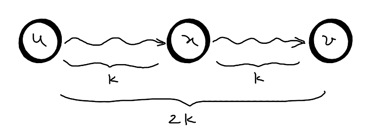
The idea is quite simple: if we know all the shortest paths for any \((u,v)\) using at most \(k\) edges, then the shortest paths for any \((u,v)\) using at most \(2k\) edges is the minimum sum of pair of paths using at most \(k\) edges among all possible predecessors of \(v\). For clarity see the picture below:

/* Repeated squaring: in the absence of negative cycles d:k = d:m for any k >= n - 1,
 * so we can compute d:n-1 within ceil(log(n-1)) loops.
 */
for(int k = 1; k < n - 1; k*=2) { // at most 2*k edges

	for (int u = 0; u < n; u++) {
		for (int v = 0; v < n; v++) {

			for (int x = 0; x < n; x++) { // all predecessors of v
				if (d[u][x] == INF || d[x][v] == INF) continue; // no paths

				d[u][v] = min(d[u][v], d[u][x] + d[x][v]);
			}
		}
	}
}
Path Reconstruction
Path reconstruction is very simple (and similar with the one from the first implementation):
- \(pred[u][v] = x \rightarrow pred[u][v] = pred[x][v]\);
- \(next[u][v] = next[u][x] \rightarrow next[u][v] = next[u][x]\);
Complexity
Time complexity is: \(T(V, E) = O(V^3log(n))\), and the auxiliary space complexity \(S(V,E) = O(V^2)\).
Negative Cycle Detection
Just as plain Bellman-Ford, Generalized Bellman-Ford also detects negative cycles. If a shorter path exists after computing \(log(n)\) square distance matrices, then the graph must contain a negative cycle, which basically means that there is a loop from \(v\) to \(v\) that is less than \(0\), so the distance matrix must contain some value less than \(0\) on its diagonal.